40 (advanced analysis) the equation for the demand curve in the below diagram
Demand Curve => ↑ QD and ↑P QD = a + bP + cY QS = d + eP Let, QD = 200 -2P + ½Y QS = 3P - 100 Given the above Demand and Supply functions, what is the impact on the Market Equilibrium of Y increasing from 0 to 20? 20. Which of the following equations represents the saving schedule implicit in the above data? A) S = C - Yd B) S = 40 + .4Yd C) S = 40 + .6Yd D) S = -40 + .4Yd Answer: D 21. Other things equal, a decrease in the real interest rate will: A) shift the investment demand curve to the right. B) shift the investment demand curve to the left.
(Advanced analysis) Assume the equation for the total demand for money is L = 0.4Y + 80 Picture 4 i, where L is the amount of money demanded, Y is gross domestic product, and i is the interest rate. If gross domestic product is $200 and the interest rate is 10 (percent), what amount of money will society want to hold? a. $200 b. $120 c. $320 d ...

(advanced analysis) the equation for the demand curve in the below diagram
The slope of the demand curve and the Demand Equation. Demand Equation. Demand equation can be written as , Qd= a- bP. a- is the point that represent the value for Qd (quantity) when P (Price) = 0. b - ∆Qd/ ∆P. Slope of the Demand curve. The slope of the any straight line curve can be found by the following formula. View 4.png from MATHEMATIC 101 at American University in Cairo. 15. "M m . Q5" "'1" (Advanced analysis) The equation for the demand curve in the above diagram: a. Is P=70-Q. b. Is P=35-20. C. (Advanced analysis) The equation for the demand curve in the below diagram: is P = 35 - .5Q. The construction of demand and supply curves assumes that the primary variable influencing decisions to produce and purchase goods is: price.
(advanced analysis) the equation for the demand curve in the below diagram. The demand curve D0 and the supply curve S0 show that the original ... Figure 2 and the text below illustrates using the four-step analysis to answer this ... A Decrease in Demand. Panel (b) of Figure 3.10 "Changes in Demand and Supply" shows that a decrease in demand shifts the demand curve to the left. The equilibrium price falls to $5 per pound. As the price falls to the new equilibrium level, the quantity supplied decreases to 20 million pounds of coffee per month. 7.1 MODEL EQUATIONS ... The supply and demand curves which are used in most ... The following descriptions of supply and demand assume a ... Equilibrium: Where Supply and Demand Intersect. When two lines on a diagram cross, this intersection usually means something. On a graph, the point where the supply curve (S) and the demand curve (D) intersect is the equilibrium.The equilibrium price is the only price where the desires of consumers and the desires of producers agree—that is, where the amount of the product that consumers ...
Economics questions and answers. (Advanced analysis) The equation for the demand curve in the below diagram 30 20 5 10 D о 0 to 40 20 60 Multiple Choice Email is P= 70 - Is P=35-20 Is P-35-50. Consumer surplus is everything above the price and below the demand curve. Before the price supports are enacted, this is areas A, B and E above. This is a triangle with a base of 20 and a height of 10 (=12-2). Thus, the area of this triangle, and thus the consumer surplus, equals 0.5(20)(10) = $100. Description: 8 edition. — Pearson, 2013. — 323 pages. This file contains Teaching Notes and Solution Manual for the 8th Edition of Pindyck R., Rubinfeld D. Microeconomics, published by Pearson Education in 2012. For undergraduate and graduate function could be the following linear equation for a small town's per- household ... to pay any price at or below the demand curve (indicated by ↓), and ...
Ο Ο P=4 + 0.50. · Price Q, QQ, Quantity Demanded Refer to the diagram. In the P1P2 price range, demand is Multiple Choice relatively elastic perfectly elastic 0 ... (Advanced analysis) The equation for the demand curve in the diagram shown. is P = 35 − .5Q. One reason that the quantity demanded of a good increases when its price falls is that the (Advanced analysis) The equation for the demand curve in the above diagram: A) is P = 70 - Q. B) is P = 35 - 2Q. C) is P = 35 - .5Q. D) cannot be determined from the information given. a) Consumer surplus is equal to the area under the demand curve. b) Producer surplus is equal to the area under the supply curve. c) Both producer and consumer surplus are equal to price multiplied by quantity. d) None of the above statements is true. 6. Consider the supply and demand curve diagram below. If the price of this good is $6, then:
Chap006App - Chapter 06 Consumer Behavior(Appendix Chapter ...
Equation (1.5) and (1.6) are the demand curves for capital and labour. ... 15For a more precise analysis, one could use the phase diagram of ...

Eckhard Bick - PDF Free Download
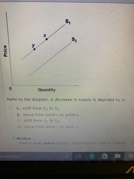
(Advanced analysis) The equation for the demand curve in the below diagram: is P = 35 - .5Q. Refer to the diagram. A decrease in demand is depicted by a.

Economics 848 – Coursepaper.com
Drawing a Demand Curve. The demand curve is based on the demand schedule. The demand schedule shows exactly how many units of a good or service will be purchased at various price points. For example, below is the demand schedule for high-quality organic bread: It is important to note that as the price decreases, the quantity demanded increases.
Module 5: Individual Demand and Market Demand – Intermediate Microeconomics
Plug QM = 10 into demand equation, we have P M = -10 + 40 = $30 f) Suppose this market was a perfectly competitive market (i.e., the monopolist's demand curve is still the market demand curve, but now there are many firms providing gas for the market). Given the
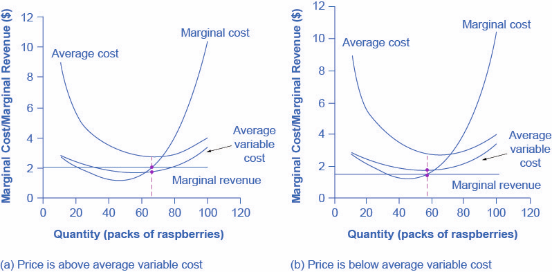
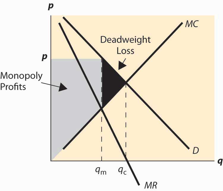
Understanding Profit
to apply to movements along the supply curve. The Demand Curve. The . demand curve. shows how much of a good consumers are willing to buy as the price per unit changes. We can write this relationship between quantity demanded and price as an equation: Q. D = Q. D (P) or we can draw it graphically, as in Figure 2.2. Note that the demand curve in ...

Solved: 1. Elasticities: Consider the following supply and ...
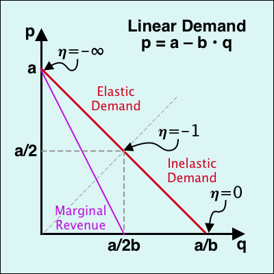
demand curve is the change in price divided by the change in quantity. For example, a decrease in price from 27 to 24 yields an increase in quantity from 0 to 2. Therefore, the slope is − 3 2 and the demand curve is P = 27 −1.5Q. The marginal revenue curve corresponding to a linear demand curve is a line with the same intercept as the ...
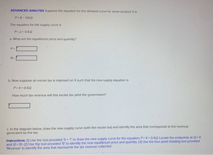
Solved: ADVANCED ANALYSIS Suppose The Equation For The Dem ...
This full solution covers the following key subjects: . This expansive textbook survival guide covers 27 chapters, and 532 solutions. Microeconomics was written ...

Government Intervention - Producer Subsidies | Economics ...
Transcribed image text: (Advanced analysis) The equation for the demand curve in the diagram shown. P 30- 20 10+ + o O 20 40 60 Multiple Choice Multiple Choice is P=35-20 is P=70-Q is P= 35 - .5Q. cannot be determined from the information given.
Note in the diagram that the shift of the demand curve, by causing a new equilibrium price to emerge, resulted in movement along the supply curve from the ...
Indifference Curves
(Advanced analysis) Answer the question on the basis of the following information. The demand for commodity X is represented by the equation P = 10 - 0.2Q and supply by the equation P = 2 + 0.2Q. Refer to the above information. If demand changed from P = 10 - .2Q to P = 7 - .3Q, the new equilibrium quantity is:
Using bio-oils for improving environmental performance of an advanced resinous binder for pavement applications with heat and noise island mitigation potential - ScienceDirect
(Advanced analysis) The equation for the demand curve in the below diagram: ... (Advanced analysis) Answer the question on the basis of the following information. The demand for commodity X is represented by the equation P = 100 - 2Q and supply by the equation P = 10 + 4Q.
Hicksian and Marshallian Demands | SpringerLink
Demand: P=10-0.2Qd. Supply: P=2+0.2Qs. Putting the supply and demand curves from the previous sections together. These two curves will intersect at Price = $6, and Quantity = 20. In this market, the equilibrium price is $6 per unit, and equilibrium quantity is 20 units. At this price level, market is in equilibrium.
31 Given The Cost Curves In The Diagram, What Market ...
3-16 Advanced analysis: Assume that the demand for a commodity is represented by the equation P = 10 .2Qd and supply by the equation P = 2 + .2Qs, where Qd and Qs are quantity demanded and quantity supplied, respectively, and P is price. Using the equilibrium condition Qs = Qd, solve the equations to determine equilibrium price.
The Global Food System: analysing the trends, impacts and solutions
Generating the Aggregate Demand Curve. The IS-LM model studies the short run with fixed prices. This model combines to form the aggregate demand curve, which is negatively sloped; hence when prices are high, demand is lower. Therefore, each point on the aggregate demand curve is an outcome of this model.
The virtues of negative exponential demand
Its supply curve is S = 20+20P. Derive and graph Home's import demand schedule. What would the price of wheat be in the absence of trade? Import demand is given by the equation MD(P) = S(P) − D(P) = 80 − 40P. The absence of trade is the equivalent to import demand being zero, which happens at P = 2. The graph is seen below.

Drug Channels: Utilizing Gini Coefficient To Anticipate ...
Transcribed image text: (Advanced analysis) The equation for the supply curve in the below diagram is approximately 30- -Q Ο 20 40 60 80 100 Multiple Choice Ο P= 4 - 30. Ο P= 4 + 0.30. Ο Ο P=4 + 20. Ο Ο P=4 + 0.50. · Price Q, QQ, Quantity Demanded Refer to the diagram. In the P1P2 price range, demand is Multiple Choice relatively elastic perfectly elastic 0 relatively inelastic. 0 of ...

Microeconomics 19th Edition Quiz 180 - ExamABC
demand and supply on the world markets as −0.25 for demand and 0.5 for supply. Assume that steel has linear demand and supply curves throughout. (a) (10 points) Solve for the equations of demand and supply in this market and sketch the demand and supply curves. Assume that this is a competitive market and assume that demand and supply are linear.
II: General Concepts and Issues in: Tax Policy Handbook
Suppose the demand curve facing a monopoly firm is given by Equation 10.1, where Q is the quantity demanded per unit of time and P is the price per unit: Equation 10.1. Q = 10 −P Q = 10 − P. This demand equation implies the demand schedule shown in Figure 10.4 "Demand, Elasticity, and Total Revenue".

PPT - Market Equilibrium PowerPoint Presentation, free ...
The above demand schedule which has been derived from the indifference curve diagram can be easily converted into a demand curve with price shown on the V-axis and quantity demanded on the X-axis. It is easier to understand the derivation of demand curve if it is drawn rightly below the indifference curve diagram.
Factors that Affect the Market Demand Curve - Video & Lesson Transcript | Study.com
(Advanced analysis) The equation for the demand curve in the below diagram: is P = 35 - .5Q. The construction of demand and supply curves assumes that the primary variable influencing decisions to produce and purchase goods is: price.

MicroEconomic 443 | Coursepaper.com
View 4.png from MATHEMATIC 101 at American University in Cairo. 15. "M m . Q5" "'1" (Advanced analysis) The equation for the demand curve in the above diagram: a. Is P=70-Q. b. Is P=35-20. C.
Unit 9 The labour market: Wages, profits, and unemployment – The Economy
The slope of the demand curve and the Demand Equation. Demand Equation. Demand equation can be written as , Qd= a- bP. a- is the point that represent the value for Qd (quantity) when P (Price) = 0. b - ∆Qd/ ∆P. Slope of the Demand curve. The slope of the any straight line curve can be found by the following formula.

Answer According to the law of demand if the demand curve ...
Sustainable irrigation based on co-regulation of soil water supply and atmospheric evaporative demand | Nature Communications

Assume the following Keynesian model for the economy of ...
Module 5: Individual Demand and Market Demand – Intermediate Microeconomics
Indifference Curves
II: General Concepts and Issues in: Tax Policy Handbook
Refer To The Diagram An Increase In Quantity Supplied Is ...
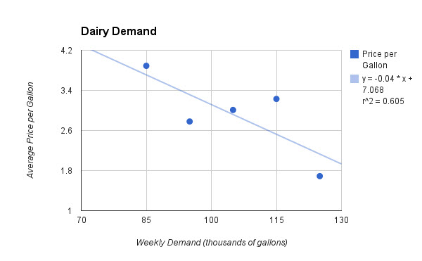
Regression Using Google Sheets | PBL Pathways
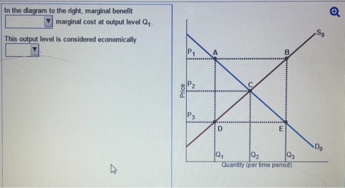
Refer To The Diagram At Output Level Q1 - Free Diagram For ...
Supply and demand - Wikipedia
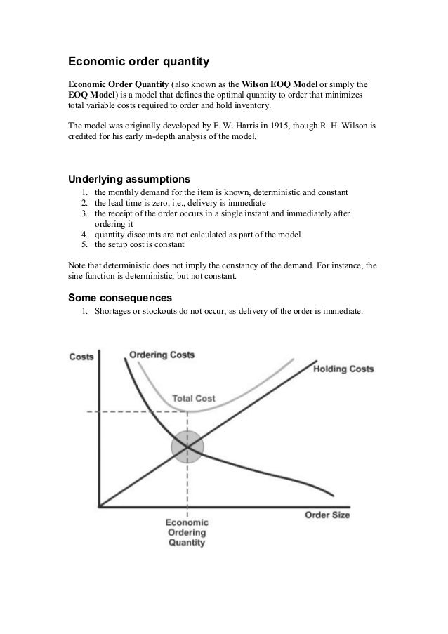
Economic order quantity
15.2: Basic Analysis - Social Sci LibreTexts
Module 5: Individual Demand and Market Demand – Intermediate Microeconomics
Marginal Analysis & Profit Maximization - ECON 101: THE BASICS

(Advanced analysis) The equation for the supply curve in ...
The impact of China's import ban: An economic surplus analysis of markets for recyclable plastics - ScienceDirect

(Advanced analysis) The equation for the supply curve in ...
Economic Models
0 Response to "40 (advanced analysis) the equation for the demand curve in the below diagram"
Post a Comment